You’ve probably heard the mantra of modern artificial intelligence: make it bigger. Bigger models, more data, more computing power. But why does this actually work? It’s not just brute force; it’s a predictable mathematical relationship known as scaling laws. These empirical rules describe how a neural network’s performance improves as you increase its size or training resources.
For years, building large language models felt like gambling. Training runs cost millions and took months. If you guessed wrong about the architecture or data mix, you lost everything. Scaling laws changed that. They turned a high-stakes gamble into a calculated investment. By understanding these laws, researchers can predict exactly how much better a model will get if they double its parameters or triple the training data. This article breaks down why more parameters improve performance, how these predictions are made, and what the latest research from 2025 and 2026 tells us about the future of AI efficiency.
The Core Mechanism: Power Laws and Predictable Improvement
At the heart of scaling laws is a simple but powerful concept: the power law. In physics and economics, power laws describe relationships where one quantity varies as a power of another. In AI, this means that as you increase the number of parameters (the internal knobs and dials a model adjusts during learning), the error rate-or "loss"-drops in a smooth, predictable curve.
Think of it like filling a bucket with water. At first, adding water makes a big difference in the level. As the bucket gets fuller, each additional cup adds less height, but the trend remains consistent. Similarly, increasing model parameters leads to steady decreases in test loss. Foundational research has shown that this relationship holds true across seven orders of magnitude. That means whether you’re doubling a small model or expanding a massive one by a factor of ten million, the improvement follows the same mathematical pattern.
This predictability is revolutionary. Before scaling laws, engineers had to train multiple versions of a model to see which worked best. Now, they can train smaller, cheaper versions, fit a power-law curve to the results, and extrapolate the performance of a much larger model. This approach reduces computational requirements by up to 10,000 times. For example, the performance of GPT-4 was largely predicted using these power-law relationships between compute and test loss before the final, expensive training run even began.
Why More Parameters Actually Help
It’s tempting to think that more parameters just mean the model memorizes more facts. While capacity increases, the real benefit is efficiency. Larger models make better and more efficient use of available information and context than smaller ones. This isn’t about rote memory; it’s about nuanced understanding.
Consider few-shot learning, where a model answers questions based on a few examples provided in the prompt. Smaller models often struggle here, failing to generalize from limited examples. However, as demonstrated by GPT-3, larger models show significant improvements in few-shot learning. They don’t just recognize patterns; they infer underlying structures. The improvement is smooth, not sudden. There are no magic thresholds where a model suddenly becomes "smart." Instead, capabilities emerge gradually as scale increases, allowing reliable extrapolation across different sizes.
This smooth improvement characterizes scaling law behavior. It allows researchers to trust that if a small model shows promise, a larger version will likely excel. This insight underpins the entire strategy of modern foundational tech development. It shifts the focus from architectural guesswork to resource allocation. The question changes from "Will this architecture work?" to "How much compute do we need to reach our target performance?"
Three Types of Scaling Laws in Modern Research
As AI has evolved, so have the metrics used to measure success. Recent contributions, including a notable 2025 NeurIPS paper, identified three distinct types of scaling laws that help researchers predict performance more accurately:
- Compute Scaling: This measures performance against the total amount of computation used (floating-point operations). It stabilizes over approximately 1.5 to 2.5 orders of magnitude in its final ranges.
- Parameters-Plus-Tokens Scaling: This combines the number of model parameters with the number of training tokens (words or subwords). It offers a balanced view of model capacity versus data exposure.
- Gold Reference Likelihood Scaling: This evaluates how likely the model is to generate the correct reference answer. It stabilizes over a broader range of approximately five orders of magnitude, making it highly reliable for long-term predictions.
All three perform comparably in predictive accuracy, but they offer different insights. Compute scaling is crucial for budgeting, while gold reference likelihood helps assess quality control. Generative evaluations introduce new hyperparameters that researchers can tweak to control these scaling law parameters, enhancing the predictability of performance outcomes.
Architectural Optimization: Beyond Just Size
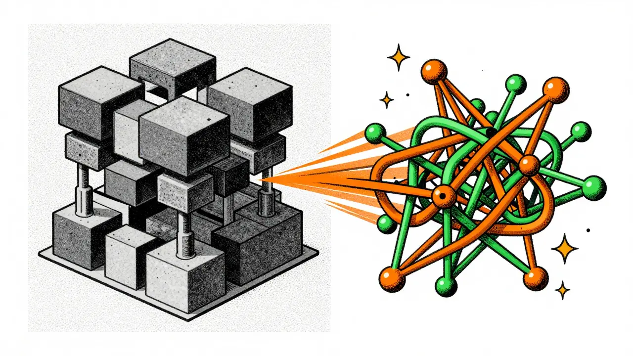
Historically, scaling laws treated architecture as a fixed variable. You’d pick a transformer design and scale it up. However, recent advancements have integrated architectural optimization directly into scaling laws. Researchers trained over 200 models ranging from 80 million to 3 billion parameters, using datasets of 8 billion to 100 billion tokens. This allowed them to develop "conditional scaling laws" that predict optimal architectural choices for specific scales.
The results were striking. Under identical training budgets, optimized architectures achieved up to 2.1 percent higher accuracy and 42 percent greater inference throughput compared to standard baselines like LLaMA-3.2. Specifically, a Panda-1B model trained on 100 billion tokens outperformed the LLaMA-3.2-1B baseline by an average of 2.1 percent across downstream tasks. Meanwhile, a Panda-3B variant delivered 42 percent higher inference throughput than LLaMA-3.2-3B while maintaining superior accuracy.
This integration marks a significant evolution. It means that scaling isn’t just about throwing hardware at a problem. It’s about designing the right shape for the model size. Conditional scaling laws enable researchers to select network architecture parameters that maximize performance for specific scale targets, ensuring that every parameter counts.
| Feature | Standard Baseline (e.g., LLaMA-3.2) | Optimized Architecture (e.g., Panda Series) |
|---|---|---|
| Accuracy Improvement | Baseline | +2.1% average across tasks |
| Inference Throughput | Baseline | +42% faster processing |
| Training Tokens | Variable | Optimized for 8B-100B tokens |
| Parameter Range | Fixed architecture | Conditional optimization (80M-3B params) |
Challenging Old Assumptions: Small Models vs. Large Models
For a long time, there was a belief that small models and large models behaved fundamentally differently. The assumption was that scaling laws derived from giant models wouldn’t apply to smaller ones, and vice versa. However, recent MIT-IBM research challenged this view. By analyzing models ranging from 70 million to 17 billion parameters trained on datasets exceeding one trillion tokens, they found strong correlations across all sizes.
Unexpectedly, scaling laws fitted to large models could accurately predict the performance of smaller models. One researcher noted, "If they're totally different, they should have shown totally different behavior, and they don't." This finding democratizes access to advanced AI techniques. Organizations with limited computational resources can now use insights from large-scale research to optimize their smaller models effectively.
The study also revealed that only three of five key hyperparameters explain nearly all variation in model behavior. This simplification makes scaling law estimation more efficient, reliable, and accessible for AI researchers working under varying budget constraints. It suggests that the complexity of AI development might be more manageable than previously thought, provided you know which levers to pull.

Practical Applications: Resource Allocation and Decision Making
So, how do you use scaling laws in practice? They serve as a strategic compass for AI development. Here are the primary jobs-to-be-done that scaling laws address:
- Performance Prediction: Estimate how model performance will improve with additional data, larger models, or increased compute. This helps set realistic expectations for stakeholders.
- Resource Allocation: Determine whether it’s more cost-effective to add parameters, gather more data, or invest in better hardware. Scaling laws provide the ROI calculation for each option.
- Model Design Optimization: Decide whether to prioritize increased model size, additional training data, or improved training techniques. Conditional scaling laws guide architectural choices.
- Risk Mitigation: Reduce the financial risk of large-scale pretraining by validating configurations on smaller models first. This prevents costly failures in production environments.
Organizations use these laws to justify continued investment in AI research. They provide confidence in expensive training runs and ensure that resources are allocated efficiently. Whether you’re a startup with a limited GPU cluster or a tech giant with thousands of TPU cores, scaling laws offer a universal framework for decision-making.
Limitations and Future Directions
While powerful, scaling laws are not infallible. Predicting larger model performance from smaller models remains difficult and can be inaccurate. Models may behave differently depending on scale, especially when crossing certain thresholds of capability. Additionally, the quality of training data plays a critical role. Scaling laws assume sufficient, high-quality data; if the data is noisy or biased, increasing parameters won’t necessarily improve performance-it might just amplify errors.
Current research focuses on incorporating architectural considerations alongside traditional scaling dimensions. The conditional scaling law framework shows that optimal architectural configurations vary predictably with model size. This integration represents a significant evolution from earlier formulations that treated architecture as relatively fixed. As we move forward, expect to see more nuanced scaling laws that account for data quality, energy efficiency, and real-time inference costs.
What are scaling laws in AI?
Scaling laws are empirical relationships that describe how neural network performance changes as key factors like model size, dataset size, and compute are scaled up. They typically follow a power-law distribution, allowing researchers to predict performance improvements based on resource investments.
Why do more parameters improve model performance?
More parameters allow models to capture more complex patterns and nuances in data. Larger models make better and more efficient use of available information, leading to smoother improvements in tasks like few-shot learning and general reasoning, rather than just memorization.
Can scaling laws predict the performance of small models?
Yes. Recent MIT-IBM research showed that scaling laws fitted to large models can accurately predict the performance of smaller models. This challenges the previous assumption that small and large models behave fundamentally differently.
What is the difference between compute scaling and parameters-plus-tokens scaling?
Compute scaling measures performance against total computational operations, useful for budgeting. Parameters-plus-tokens scaling combines model size with data volume, offering a balanced view of capacity versus exposure. Both stabilize over different ranges but provide comparable predictive accuracy.
How do conditional scaling laws help with architecture?
Conditional scaling laws predict optimal architectural choices for specific model sizes. By integrating architecture into the scaling equation, researchers can design models that achieve higher accuracy and throughput under identical training budgets, as seen in comparisons with LLaMA-3.2.