Imagine you are building a customer support chatbot. A user types a question and hits enter. If the screen stays blank for six seconds before a single word appears, the user assumes the system is broken. They click away. This split-second judgment defines the life or death of your interactive large language model application. The difference between a tool people love and one they abandon often comes down to milliseconds. To keep users engaged, you need to set strict latency budgets. These budgets define exactly how long your system can take to respond before the experience feels sluggish.
Setting these limits isn't just about picking a fast server. It requires understanding the hidden mechanics of how models process text. You have to balance speed, cost, and intelligence. In this guide, we will break down the math behind responsiveness, explore the trade-offs in model architecture, and show you how to engineer systems that feel instant.
The Anatomy of LLM Latency
To control latency, you first need to know where it hides. Large language models do not generate text like a human typing on a keyboard. They operate in two distinct phases, each with different bottlenecks. Understanding this split is crucial for setting realistic expectations.
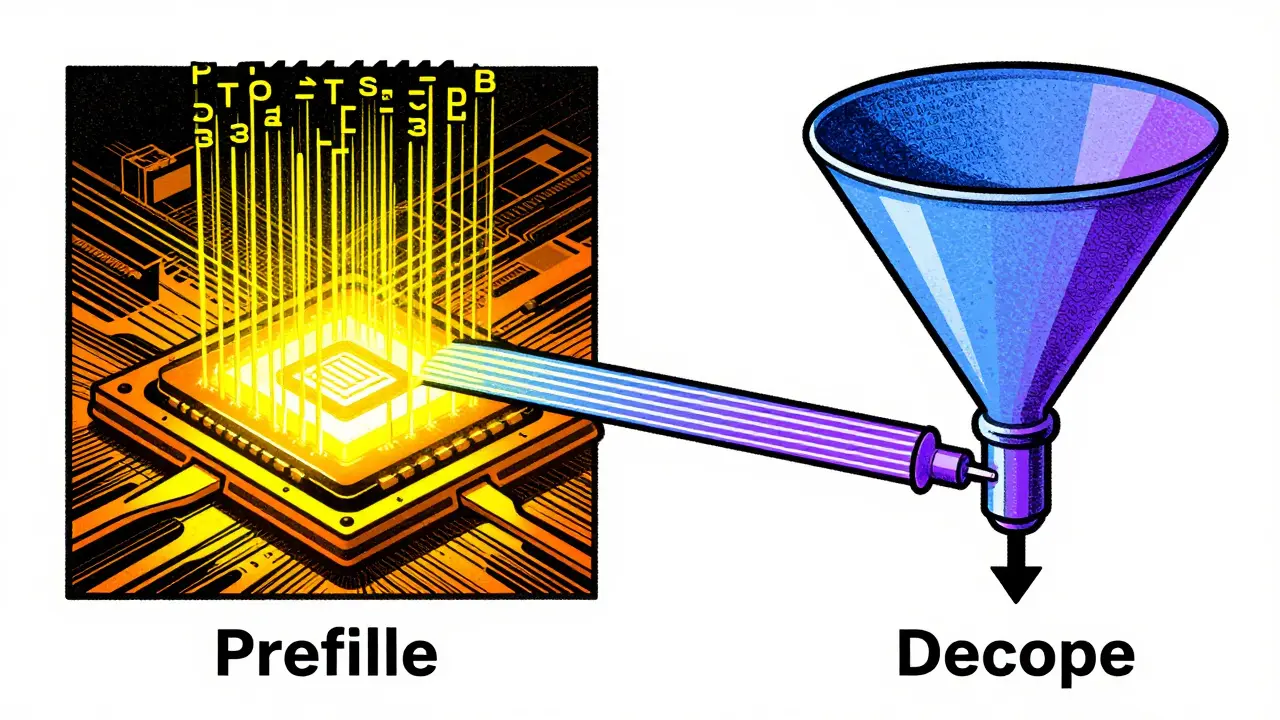
The first phase is called prefill. When a user sends a prompt, the model reads the entire input at once. It builds a memory structure known as the Key-Value (KV) cache. This step is compute-bound, meaning it relies heavily on the processing power of the GPU. Because the model processes all input tokens in parallel, this phase is generally fast, unless the input context is massive.
The second phase is decode. Here, the model generates the response token by token. Each new word depends on the previous ones. This creates a sequential bottleneck. Unlike the prefill phase, decode is memory-bound. The speed limit here is not how fast the GPU calculates numbers, but how quickly it can move data from memory to the processor. As the conversation grows, the KV cache gets larger, making each subsequent token slightly harder to retrieve. This asymmetry means that while short answers might fly out, long explanations can drag down the perceived speed.
Defining Your Metrics: TTFT vs. Throughput
When engineers talk about speed, they often confuse two very different metrics. For an interactive app, you must track both, but they serve different purposes.
- Time to First Token (TTFT): This measures the delay between the user hitting "Enter" and seeing the first character appear. TTFT is dominated by the prefill phase. If your TTFT is high, the user waits in silence. Research shows that if TTFT exceeds two to three seconds, user satisfaction drops sharply. This is your primary metric for "responsiveness."
- Tokens Per Second (TPS): This measures how fast the rest of the sentence streams in after the first token. TPS is dominated by the decode phase. If your TPS is low, the text trickles out slowly. Users can tolerate lower TPS better than high TTFT because they see progress immediately.
Your latency budget should prioritize TTFT. A target of under 1000 milliseconds for TTFT is standard for high-quality interactive experiences. Once the first token arrives, you can aim for 20 to 50 tokens per second to ensure the full answer completes quickly. If you optimize only for total completion time, you might sacrifice TTFT, leaving users staring at a blank screen.
The Batching Trap: Speed vs. Cost
A common strategy to reduce costs is batching. Instead of processing one request at a time, the server groups multiple requests together. This keeps the GPU busy and improves efficiency. However, batching introduces a dangerous trade-off for interactive apps.
Consider the Qwen 2.5 7B model. When running with a batch size of 1, the latency is roughly 976 milliseconds. Increase the batch size to 8, and the latency per request drops significantly in terms of throughput efficiency, but individual wait times can spike due to queueing. More importantly, as you increase the number of concurrent sequences (max_num_seqs), the GPU memory fills up faster. The system spends more time managing the queue and less time generating tokens.
| Batch Size | Avg Latency (ms) | Throughput Gain | User Experience Impact |
|---|---|---|---|
| 1 | 976 ms | Baseline | Predictable, low jitter |
| 8 | ~126 ms (per token) | High | Risk of increased TTFT under load |
| 32+ | Variable | Diminishing returns | High risk of timeout errors |
If your application handles casual queries, small batches work well. But for real-time interactions where every millisecond counts, aggressive batching can ruin the experience. You must cap your batch sizes dynamically based on current load to protect TTFT.
Architectural Levers: Speculative Decoding and Quantization
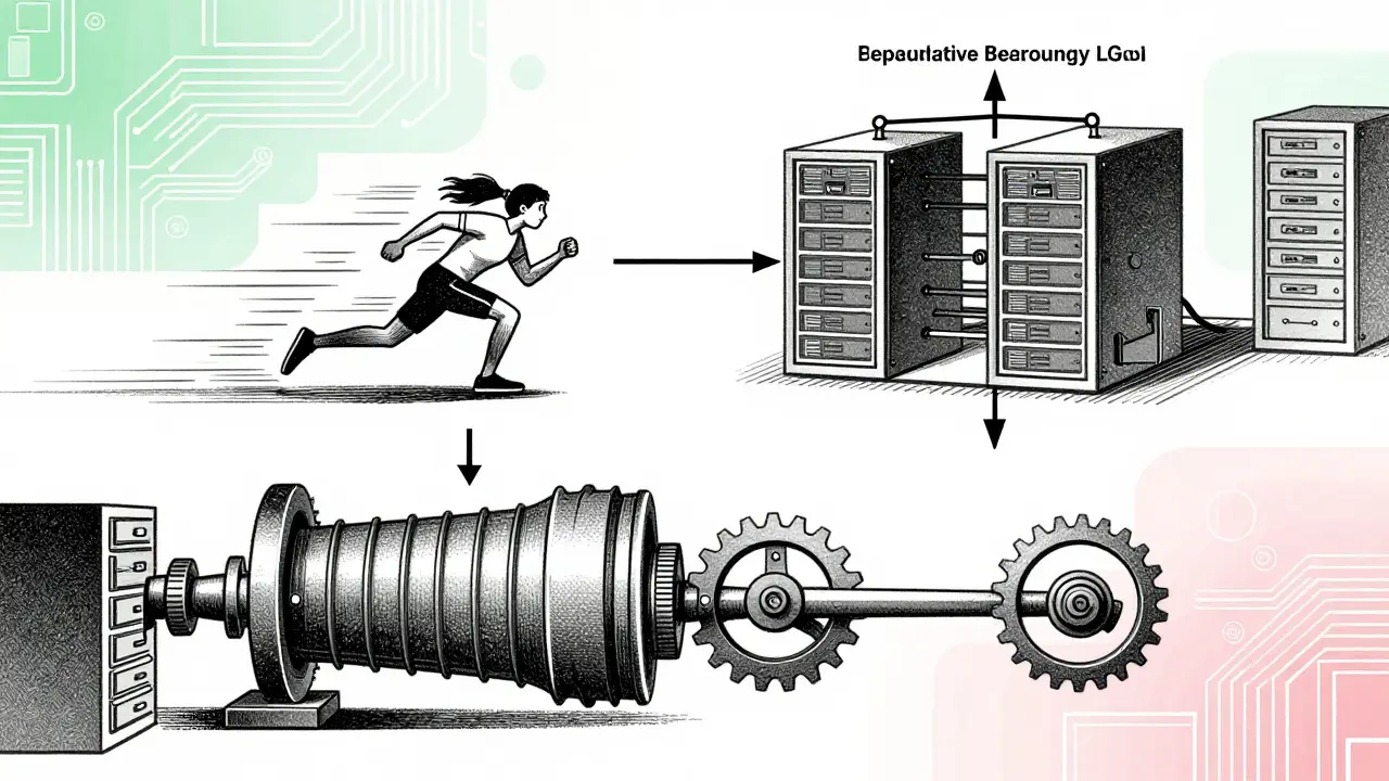
When hardware alone cannot meet your latency budget, you need architectural tricks. Two techniques stand out: speculative decoding and quantization.
Speculative decoding uses a smaller, faster "draft" model to predict several tokens ahead. The larger, smarter model then verifies these predictions in parallel. If the draft is correct, you save significant time. This technique can reduce inference latency by 2x to 4x. It is particularly effective for reasoning-heavy tasks where the larger model would otherwise stall. The trade-off is extra compute overhead for the draft model, but the net gain in speed usually justifies the cost.
Quantization reduces the precision of the model's weights. For example, converting a model from BF16 (16-bit floating point) to MXFP4 (4-bit mixed precision) drastically shrinks its memory footprint. The GPT OSS 20B model, using MXFP4, requires only about 13.1 GB of GPU memory. Smaller models fit into faster memory tiers and allow higher batch sizes without hitting capacity limits. While extreme quantization can hurt accuracy, modern methods preserve quality surprisingly well while boosting speed.
Model Selection and Hardware Constraints
Your choice of model dictates your baseline latency. A 109-billion parameter model requires three NVIDIA H100 GPUs to run efficiently. A 400-billion parameter model needs at least ten such GPUs. These infrastructure costs directly impact latency because larger models have longer critical paths for computation.
Smaller models, like those with 8 billion parameters, can run on a single 80GB GPU. They offer much lower TTFT and higher TPS. For many interactive use cases, an 8B model paired with good prompting strategies outperforms a slower 70B model. If you need the reasoning power of a large model, consider using a Mixture of Experts (MoE) architecture. Models like GPT OSS 20B MoE activate only a fraction of their parameters per pass (e.g., 3.6B active parameters). This sparsity allows them to run faster than dense models of similar size, though routing overhead adds complexity.
Implementing Caching Strategies
The fastest request is the one you never process. Caching frequently asked questions or common RAG (Retrieval-Augmented Generation) contexts can eliminate latency entirely for repeat queries. In online RAG applications, prompts can be huge (up to 10,000 tokens). Processing this prefill repeatedly is expensive and slow.
Implement a semantic cache that stores embeddings of user queries along with responses. If a new query matches a cached entry above a certain similarity threshold, return the stored answer instantly. Be careful with invalidation; stale information is worse than slow information. Use time-to-live (TTL) policies or version tags to ensure cached data remains accurate.
Building a Realistic Latency Budget
So, what does a practical budget look like? Let's create a scenario for a startup handling 10,000 requests per day with an online RAG system.
- Set the TTFT Target: Aim for < 800ms. This ensures the UI updates almost instantly.
- Define TPS Minimum: Require > 30 tokens/sec. This keeps the reading flow natural.
- Select Model Tier: Start with an 8B parameter model for general queries. Route complex, high-value queries to a 70B+ model using a classifier.
- Apply Optimization: Enable speculative decoding for the large model tier. Use FP8 or INT8 quantization for the small model.
- Monitor P95 Latency: Do not optimize for averages. Track the 95th percentile. If 5% of users wait 10 seconds, your product fails.
This approach balances cost and performance. Using a 109B model for every query might cost $15,000 per month and still struggle with latency under load. By mixing models and optimizing the path, you can maintain sub-second responsiveness while keeping costs manageable.
What is a good Time to First Token (TTFT) for an LLM app?
Aim for under 1000 milliseconds. Ideally, keep it below 500ms for a truly instant feel. Anything over 2-3 seconds causes users to perceive the app as unresponsive or broken.
How does batching affect interactive latency?
Batching increases throughput but can increase latency for individual requests. Requests wait in a queue until the batch is full. For interactive apps, use dynamic batching with strict caps to prevent excessive wait times.
Is speculative decoding worth the complexity?
Yes, especially for large models. It can reduce latency by 2-4x by allowing the model to verify multiple tokens in parallel. The added compute cost is usually lower than the cost of waiting for sequential generation.
Why is the decode phase slower than the prefill phase?
Prefill is compute-bound and parallelizable. Decode is memory-bound and sequential. Each new token requires reading the growing Key-Value cache from memory, which becomes slower as the context length increases.
How does model size impact latency budgets?
Larger models require more compute and memory bandwidth, leading to higher latency. An 8B model is typically 5-10x faster than a 70B model. Choose the smallest model that meets your accuracy requirements to maximize speed.